
Universal Sentence Encoder - Deep Learning for NLP
What is the Universal Sentence Encoder (USE)?
Google’s Universal Sentence Encoder (USE) is a tool that converts a string of words into 512 dimensional vectors. These vectors capture the semantic meaning of the sequence of words in a sentence and therefore can be used as inputs for other downstream NLP tasks like classification, semantic similarity measurement etc. A representative flow for a typical text classification task is shown below:
.png)
USE is made available publicly on TensorFlow Hub. It’s pretty easy to use:
import tensorflow_hub as hub

embed = hub.Module("https://tfhub.dev/google/"
"universal-sentence-encoder/1")
embedding = embed([
"The quick brown fox jumps over the lazy dog."])
Semantic Similarity
I realize that I’ve been casually throwing around the term ‘semantic similarity’ like it’s something you should be familiar with. It’s not. It is essentially a measure of how similar in meaning two sentences are. Sounds subjective? Let’s put some numbers on that measure. In mathematical terms, semantic similarity between two sentences is the inner product of the the sentence embeddings or sentence vectors of the two sentences. Therefore, theoretically it is a ‘score’ between -1 and 1. In most practical cases however, we observe that the score is between 0 and 1. A score closer to 1 means high similarity while that tending to 0 means no similarity. To test this and also to visualize this similarity we will look at a heatmap.
For illustrative purposes, I have picked a bunch of current (at the time of writing) news stories and grouped together headlines from different sources for the same story. The stories are taken from disparate topics like sports, technology and space exploration.

The code to generate this heatmap is given below. Feel free to play around with different sentences.
import tensorflow as tf
import tensorflow_hub as hub
import matplotlib.pyplot as plt
import numpy as np
import os
import pandas as pd
import re
import seaborn as sns

embed = hub.Module(module_url)

def plot_similarity(labels, features, rotation):
  corr = np.inner(features, features)
  sns.set(font_scale=1.2)
  g = sns.heatmap(
      corr,
      xticklabels=labels,
      yticklabels=labels,
      vmin=0,
      vmax=1,
      cmap="YlOrRd")
  g.set_xticklabels(labels, rotation=rotation)
  g.set_title("Semantic Textual Similarity")


def run_and_plot(session_, input_tensor_, messages_, encoding_tensor):
  message_embeddings_ = session_.run(
      encoding_tensor, feed_dict={input_tensor_: messages_})
  plot_similarity(messages_, message_embeddings_, 90)

headlines = [
    # Microsoft
    "Latest Windows 10 update breaks Windows Media Player, Win32 apps in general",
    "Microsoft releases cumulative update KB4469342 for Windows 10 version 1809 Release Preview Insiders",
    "Windows 10 update makes Windows Media Player almost unusable",

    # Celtics
    "Kyrie Irving highlights Marcus Smart’s play after win over New Orleans",
    "Morning sports update: What Kyrie Irving said about his 'magic' balancing video",
    "Trade Kyrie Irving? Jalen Rose Explains Why Celtics Should Consider Blockbuster",

    # Google Pixel
    "Google Pixel Slate review",
    "Google Pixel Slate review: a strong case for death of Android tablets",
    "Cam Compare: Pixel 3 XL Night Sight vs OnePlus 6T Nightscape",

    # NASA
    "NASA releases 1st clear image from InSight probe’s mission to Mars ",
    "This Mars Landing Touchdown Dance by NASA InSight Engineers Is Absolutely EPIC!",
]

similarity_input_placeholder = tf.placeholder(tf.string, shape=(None))
similarity_headline_encodings = embed(similarity_input_placeholder)
with tf.Session() as session:
  session.run(tf.global_variables_initializer())
  session.run(tf.tables_initializer())
  run_and_plot(session, similarity_input_placeholder, headlines,
               similarity_headline_encodings)
But wait…don’t get too excited just yet!
As we can see, USE is a fantastic tool and one maybe tempted to use it straight out of the box. However, it is critical to know the underlying architecture of the model and most importantly, what kind of data it was trained on. For example if you’re working with a corpus of scientific articles, it is useful to know that USE is trained on Wikipedia, which has plenty of scientific content. Thus, making the encoder an ideal choice for working with this kind of data. On the other hand, if you’re dealing with bank research reports or other kinds of business documents, USE might encounter a lot of jargon that it is unfamiliar with which may lead to erroneous results. We shall cover this later in this post.
The Universal Sentence Encoder comes in 2 flavors each with a distinct model architecture:
1. The Transformer Architecture
The Transformer based Universal Sentence Encoder constructs sentence embeddings using the encoder part of the transformer architecture proposed in this paper by Vaswani et al. On a high level, this architecture uses self-attention to compute context aware representations of words in a sentence that take into account both the ordering and identity of all the other words. These context aware word vectors are then summed up to output the vector for the entire sentence. A pictorial representation of one encoder is shown below. There are 6 such encoders stacked one on top of the other in the final model.
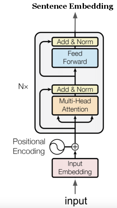
It is important to note that even though the ‘sequentiality’ (for lack of better term) of the words is taken into account in this model, we do not use any form of recurrence. This makes the model highly parallizable. If you would like to delve deeper into this cool architecture and understand its nuts and bolts under the hood, I’d recommend this awesome blog.
2. The Deep Averaging Network (DAN)
In this architecture the word embeddings for a sentence are first averaged together and then passed through a feed forward neural network as shown below.
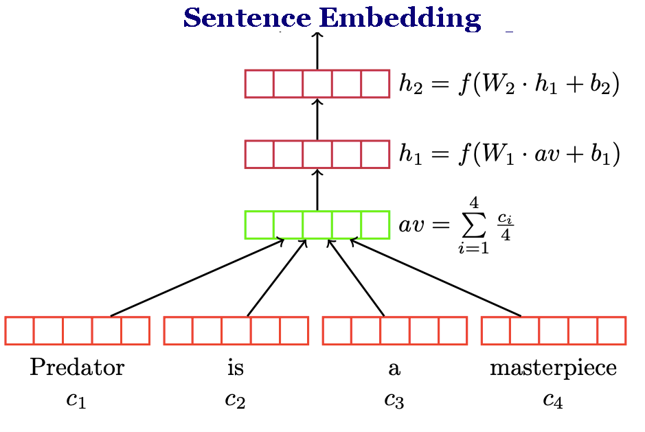
The feed forward neural network is then trained on various downstream tasks like classification, similarity etc. The main advantage of the DAN over the transformer architecture is that the compute time is linear in length of the input sequence. More information can be found in the original paper.
Choosing between the two architecture boils down to a compromise between performance and computation time. Use DAN when you need faster computation and Transformer when higher performance is a priority. However, this is just a rule of thumb. You should try using both architectures and see what works best for your application.
The Data on which USE is trained
As I had touched upon earlier, it is important to know what kind of data the encoder was trained on. This will give you an idea of what tasks USE is suitable for. I have tabulated the data and task type here:
| Task | Data |
|---|---|
| Unsupervised | Wikipedia, Web news, Web question-answer pages and discussion forums. |
| Supervised | Stanford Natural Language Inference (SNLI) corpus. |
| Transfer Learning tasks | Movie review sentiment on a 5 star scale |
| . | Sentiment of sentences mined from customer reviews |
| . | Subjectivity of sentences from movie reviews and plot summaries |
| . | Phrase level opinion polarity from news data |
| . | Fine grained question classification sourced from TREC |
| . | Binary phrase level sentiment classification |
| . | Semantic textual similarity (STS) between sentence pairs scored by Pearson correlation with human judgments |
| . | Word pairs from the psychology literature on implicit association tests (IAT) that are used to characterize model bias |
The unsupervised training entails running a Word2Vec like algorithm. Loosely speaking, just like how Word2Vec optimizes for the likelihood of a word occurring in the context of a certain window of words, USE optimizes the likelihood of a sentence in the context of its surrounding sentences. If you’re unfamiiar with Word2Vec, I’d recommend this brilliant lecture and this blog.
As you can see, a major chunk of the training text data can be classified as informal or colloquial. This should be kept in mind while dealing with applications that have text with more formal or jargon-y language.
Text Classification Example - IMDB movie review sentiment classification
We will now look at USE in action. Movie reviews from IMDB will be fed into the encoder which will convert them to fixed length 512 dimensional vectors. The vectors will then be fed into a Fully connected Neural Network. Let’s dive right in!
1. Setting up the environment:
1.1 Installing required packages
# Install the latest Tensorflow version.
!pip install --quiet "tensorflow>=1.7"
# Install TF-Hub.
!pip install tensorflow-hub
!pip install seaborn
1.2 Importing relevant libraries
import tensorflow as tf
import tensorflow_hub as hub
import matplotlib.pyplot as plt
import numpy as np
import os
import pandas as pd
import re
import seaborn as sns
from tensorflow import keras
import tensorflow as tf
import tensorflow_hub as hub
import matplotlib.pyplot as plt
import numpy as np
import os
import pandas as pd
import re
import seaborn as sns
from sklearn.model_selection import train_test_split

import keras.layers as layers
from keras.models import Model
from keras import backend as K
np.random.seed(10)
2. Downloading data and storing it as a DataFrame
# Load all files from a directory in a DataFrame.
def load_directory_data(directory):
data = {}
data["sentence"] = []
data["sentiment"] = []
for file_path in os.listdir(directory):
with tf.gfile.GFile(os.path.join(directory, file_path), "r") as f:
data["sentence"].append(f.read())
data["sentiment"].append(re.match("\d+_(\d+)\.txt", file_path).group(1))
return pd.DataFrame.from_dict(data)
# Merge positive and negative examples, add a polarity column and shuffle.
def load_dataset(directory):
pos_df = load_directory_data(os.path.join(directory, "pos"))
neg_df = load_directory_data(os.path.join(directory, "neg"))
pos_df["polarity"] = 1
neg_df["polarity"] = 0
return pd.concat([pos_df, neg_df]).sample(frac=1).reset_index(drop=True)
# Download and process the dataset files.
def download_and_load_datasets(force_download=False):
dataset = tf.keras.utils.get_file(
fname="aclImdb.tar.gz",
origin="http://ai.stanford.edu/~amaas/data/sentiment/aclImdb_v1.tar.gz",
extract=True)
train_df = load_dataset(os.path.join(os.path.dirname(dataset),
"aclImdb", "train"))
test_df = load_dataset(os.path.join(os.path.dirname(dataset),
"aclImdb", "test"))
return train_df, test_df
# Reduce logging output.
tf.logging.set_verbosity(tf.logging.ERROR)
train_df, test_df = download_and_load_datasets()
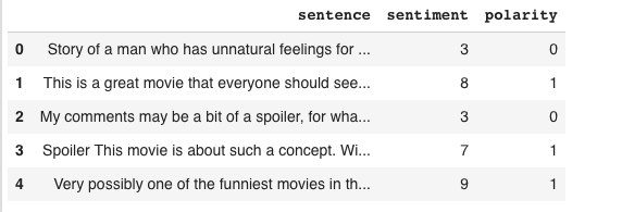
train_df.head()
Here’s what the training dataframe looks like:
train_df.head()
3. Downloading USE
https://tfhub.dev/google/universal-sentence-encoder-large/3 - corresponds to the Transformer Architecture https://tfhub.dev/google/universal-sentence-encoder/2 - corresponds to the DAN architecture
The Transformer one will be larger in size and will take longer to compute embeddings but will also provide better results. Choose the module as per your requirement and willingness to compromise between computation speed and accuracy.
module_url = "https://tfhub.dev/google/universal-sentence-encoder-large/3" #@param ["https://tfhub.dev/google/universal-sentence-encoder/2", "https://tfhub.dev/google/universal-sentence-encoder-large/3"]

embed = hub.Module(module_url)
4. Setting up the Dense Neural Network for classification
Next, we setup the a neural network as shown below. Feel free to play around with the layers and optimizer functions and other hyperparameters.
from keras.optimizers import Adam
optimizer=Adam(lr=0.001, decay=1e-4)
embed_size = 512
input_text = layers.Input(shape=(1,), dtype=tf.string)
embedding = layers.Lambda(UniversalEmbedding, output_shape=(embed_size,))(input_text)
dense1 = layers.Dense(128, activation='relu')(embedding)
dropout1 = layers.Dropout(0.1)(dense1)
pred = layers.Dense(2, activation='softmax')(dropout1)
model = Model(inputs=[input_text], outputs=pred)
model.compile(loss='binary_crossentropy', optimizer=optimizer, metrics=['accuracy'])
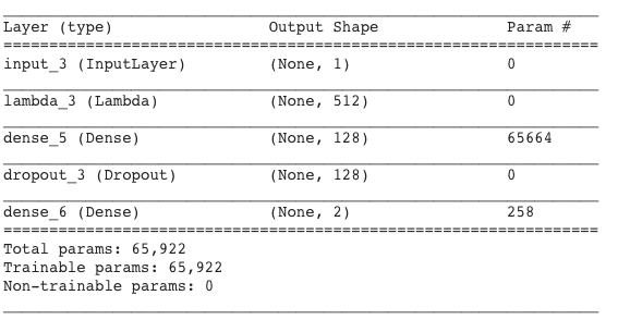
model.summary()
The model can be summarized as follows:
Now that we have the train and test dataframes, we proceed to one hot encode the labels and reshape the data. Also, we will split the training data into training and validation split. The validation data is used as the evaluation set at each step of the training. This ensures that the test data that we have is completely unseen.
train_text = train_df['sentence'].tolist()
train_text = np.array(train_text, dtype=object)[:, np.newaxis]
train_label = np.asarray(pd.get_dummies(train_df['polarity']), dtype = np.int8)

test_text = test_df['sentence'].tolist()
test_text = np.array(test_text, dtype=object)[:, np.newaxis]
test_label = np.asarray(pd.get_dummies(test_df['polarity']), dtype = np.int8)


val_text, X_test, val_label, y_test = train_test_split(test_text, test_label, stratify = test_label, random_state = 42, test_size = 0.3)
5. Training the model
with tf.Session() as session:
  K.set_session(session)
  session.run(tf.global_variables_initializer())
  session.run(tf.tables_initializer())
  history = model.fit(train_text,
            train_label,
            validation_data=(val_text, val_label),
            epochs=10,
            batch_size=250)
  model.save_weights('./imdb_dnn.h5')
Now that we can see that the model has learnt on the training data and we can use the unseen test data to evaluate the true performance of this model. This will give us an idea on how this model will generalize to new unseen data.
6. Evaluating the model on unseen Test data:
with tf.Session() as session:
  K.set_session(session)
  session.run(tf.global_variables_initializer())
  session.run(tf.tables_initializer())
  model.load_weights('./imdb_dnn.h5')
  ans = model.evaluate(X_test, y_test)


print(ans)

This show that our model accuracy is about 84.42%. Pretty good for a simple binary class classifier. However, please note that the dataset we are working with is perfectly balanced i.e. there are equal number of samples of both classes in the data. This is not the case in most real world classification tasks. For imbalanced datasets we have a variety of metrics other than accuracy to measure performance. More on that in some other post!
Conclusion
So we just used the Universal Sentence Encoder as input to a downstream text classification task. We can extend this principle to a variety of other NLP tasks that require a sentence embedding. Hope this also gave you a sneak peak into the the architecture’s basics so that the encoder is not a black box to you when you use it. Enjoy!
References
I have built this tutorial by learning from and collating blogs and examples that I found useful. Some of them are listed below: